Lab1-2. NumPy Basics for Machine Learning

Author

Byungkook Oh

Modified

2026.03.22

Objectives

Array Creation and Attributes: Create arrays and inspect shape, dtype, and ndim.
Indexing and Slicing: Select rows, columns, and subsets using slice notation and fancy indexing.
Reshaping and newaxis: Change array dimensions with reshape and insert size-1 axes with np.newaxis.
Sorting and comparison: Sort arrays and compare elements using sort, argsort, and allclose.
Vectorization: Replace slow Python loops with fast, C-optimized array operations.
Broadcasting: Perform operations on arrays of different shapes using NumPy’s shape-alignment rules.
Matrix Multiplication: Use np.matmul (the @ operator) for linear algebra.
Array Creation & Random Numbers: Initialize arrays with built-in factories and generate reproducible random data with a seeded PRNG.
Reductions: Summarize arrays along one or more axes with sum, min, max, mean, etc.
Views vs. Copies: Understand when NumPy shares memory (view) vs. allocates new data (copy) to avoid accidental mutations.

Basic Concept: Why NumPy?

In Machine Learning, we deal with massive amounts of data (vectors, matrices, tensors). Standard Python lists are too slow and memory-inefficient for these calculations. NumPy arrays are stored in contiguous blocks of memory and operations are implemented in highly optimized C code, making mathematical operations drastically faster. NumPy is the foundational library that modern deep learning frameworks (like PyTorch and TensorFlow) are built upon.

1. Array Creation and Attributes

Before we manipulate data, we need to know how to create arrays and inspect their properties.

import numpy as np

# 1-Dimensional Array (Vector)
# np.array infers the dtype from the input: integers → int64, floats → float64
a = np.array([1, 2, 3, 4, 5])
print("a =", a)
print("dtype:", a.dtype)
print("shape:", a.shape)   # tuple: (number of elements,)
print("ndim :", a.ndim)    # number of dimensions

a = [1 2 3 4 5]
dtype: int64
shape: (5,)
ndim : 1

Arithmetic operators apply element-wise — no loop required.

x = np.array([1.0, 6.0, 2.4])

print("x + 2 =", x + 2)   # add scalar to every element
print("x * 2 =", x * 2)   # multiply every element
print("x / 2 =", x / 2)   # divide every element
print("x + x =", x + x)   # add two same-shape arrays element-wise
print("x / x =", x / x)   # divide element-wise

x + 2 = [3.  8.  4.4]
x * 2 = [ 2.  12.   4.8]
x / 2 = [0.5 3.  1.2]
x + x = [ 2.  12.   4.8]
x / x = [1. 1. 1.]

Data Types (dtype)

NumPy stores all elements of an array in the same dtype. The default depends on the input literals: integer literals → int64, any float literal → float64.

y_int   = np.array([1, 4, 3])                        # no decimal → int64
y_f64   = np.array([1., 4, 3])                       # one decimal point → float64
y_f32   = np.array([1., 4, 3], dtype=np.float32)     # explicit 32-bit float

print("int64  :", y_int.dtype,  " | nbytes:", y_int.nbytes)   # 8 bytes per element
print("float64:", y_f64.dtype,  " | nbytes:", y_f64.nbytes)   # 8 bytes per element
print("float32:", y_f32.dtype,  " | nbytes:", y_f32.nbytes)   # 4 bytes per element

int64  : int64  | nbytes: 24
float64: float64  | nbytes: 24
float32: float32  | nbytes: 12

When you mix dtypes, NumPy upcasts the result to the higher-precision type so no information is lost.

z = y_f64 + y_f32     # float64 + float32 → float64
print("result dtype:", z.dtype)

result dtype: float64

Caveat: Data Types (dtype)

In deep learning, memory is expensive. Most frameworks default to float32 rather than float64. When you load data or create arrays, explicitly pass dtype=np.float32 to halve memory usage without meaningful loss in precision for gradient-based training.

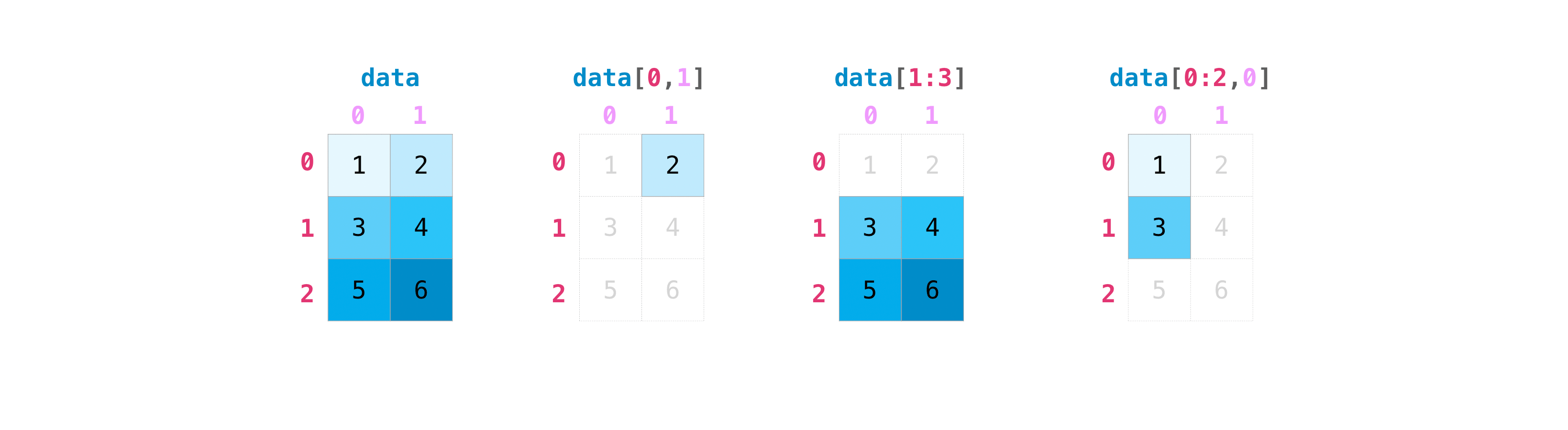
2. Indexing and Slicing

Accessing elements in NumPy is similar to standard Python lists but extends to multiple dimensions.

x = np.array([10, 20, 30, 40, 50])
print("First element:", x[0])
print("Last element:", x[-1])
print("Slice [1:4]:", x[1:4])     # Indices 1, 2, 3 (exclusive of 4)
print("Step slice [::2]:", x[::2]) # Every 2nd element from start to end

First element: 10
Last element: 50
Slice [1:4]: [20 30 40]
Step slice [::2]: [10 30 50]

M = np.arange(12).reshape(3, 4)
print("M =\n", M)
print("Specific element M[1, 2]:", M[1, 2])
print("Entire 2nd row:", M[2, :])
print("Entire 3rd column:", M[:, 3])

M =
 [[ 0  1  2  3]
 [ 4  5  6  7]
 [ 8  9 10 11]]
Specific element M[1, 2]: 6
Entire 2nd row: [ 8  9 10 11]
Entire 3rd column: [ 3  7 11]

Caveat: Slices are Views, Not Copies!

When you slice an array in NumPy, it returns a view of the original memory, not a new array. If you modify the slice, the original array is modified too. If you need an independent copy, explicitly use .copy().

x_slice = x[1:4].copy()

2D Array Indexing

The following examples use a 4×4 matrix to practise all common 2D indexing patterns.

Row and column indexing on a 2-D array. A single integer selects a row; a colon in the first position with an integer in the second selects a column.

# np.arange(1, 17) gives [1..16]; reshape(4,4) makes it 4×4; transpose flips rows/cols
A_44 = np.arange(1, 17).reshape(4, 4).transpose()
print(A_44)

[[ 1  5  9 13]
 [ 2  6 10 14]
 [ 3  7 11 15]
 [ 4  8 12 16]]

print("First row          :", A_44[0])        # single integer → selects a row
print("First col          :", A_44[:, 0])     # colon = all rows; 0 = column 0
print("Last row           :", A_44[-1])        # negative index counts from end
print("Second-to-last col :", A_44[:, -2])    # negative column index

First row          : [ 1  5  9 13]
First col          : [1 2 3 4]
Last row           : [ 4  8 12 16]
Second-to-last col : [ 9 10 11 12]

print("Rows 0–2 (A_44[0:3]):\n",              A_44[0:3])
print("\nRows 0–2, cols 1–3 (A_44[0:3, 1:4]):\n", A_44[0:3, 1:4])
print("\nRows 0–1, all cols (A_44[0:2, :]):\n",   A_44[0:2, :])

Rows 0–2 (A_44[0:3]):
 [[ 1  5  9 13]
 [ 2  6 10 14]
 [ 3  7 11 15]]

Rows 0–2, cols 1–3 (A_44[0:3, 1:4]):
 [[ 5  9 13]
 [ 6 10 14]
 [ 7 11 15]]

Rows 0–1, all cols (A_44[0:2, :]):
 [[ 1  5  9 13]
 [ 2  6 10 14]]

Fancy Indexing

Passing a list or integer array selects multiple rows at once. The result is always a copy (not a view), and indices can be repeated or in any order.

print("Rows 1 and 3:\n", A_44[[1, 3]])

Rows 1 and 3:
 [[ 2  6 10 14]
 [ 4  8 12 16]]

more_ids = np.array([3, 3, 1, 0], dtype=np.int32)
print("Repeated / unsorted rows:\n", A_44[more_ids])

Repeated / unsorted rows:
 [[ 4  8 12 16]
 [ 4  8 12 16]
 [ 2  6 10 14]
 [ 1  5  9 13]]

Fancy indexing requires integer indices

Float arrays cannot be used as indices — NumPy raises an IndexError.

row_ids_f64 = np.array([1.0, 3.0])
A_44[row_ids_f64]   # IndexError: arrays used as indices must be of integer (or boolean) type

3. Reshaping and newaxis

Machine learning code frequently needs to change an array’s shape without changing its data. Two tools cover almost every case: reshape and np.newaxis.

reshape

array.reshape(new_shape) returns a view with a different shape. The total number of elements must stay the same.

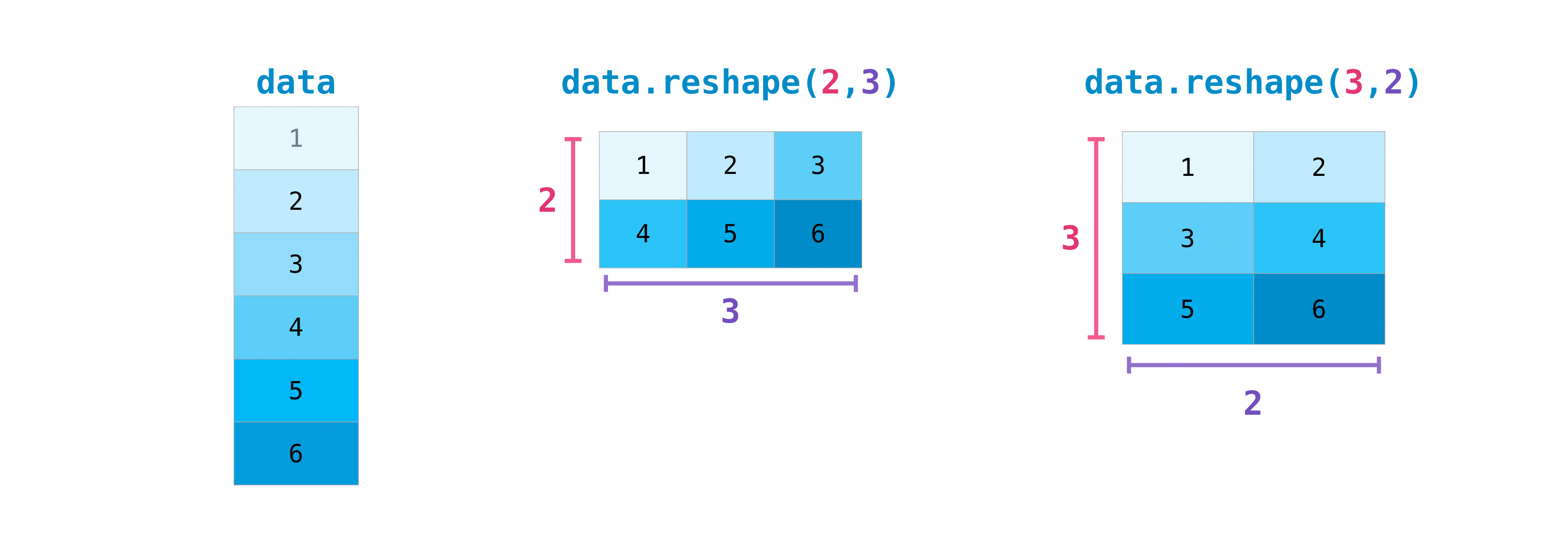
y = np.array([1.0, 4, 3])
print("y      shape:", y.shape)

y_13 = y.reshape(1, 3)    # row vector    → (1, 3)
y_31 = y.reshape(3, 1)    # column vector → (3, 1)
print("y_13 =", y_13,  " shape:", y_13.shape)
print("y_31 =\n", y_31, "shape:", y_31.shape)

y      shape: (3,)
y_13 = [[1. 4. 3.]]  shape: (1, 3)
y_31 =
 [[1.]
 [4.]
 [3.]] shape: (3, 1)

np.newaxis

np.newaxis inserts a new axis of size 1 at the chosen position — a concise alternative to reshape for adding a single dimension.

y_3   = np.array([1.0, 4, 3])
y_13  = y_3[np.newaxis, :]              # (1, 3) — row vector
y_31  = y_3[:, np.newaxis]              # (3, 1) — column vector
y_311 = y_3[:, np.newaxis, np.newaxis]  # (3, 1, 1)

print("y_13  shape:", y_13.shape)
print("y_31  shape:", y_31.shape)
print("y_311 shape:", y_311.shape)

y_13  shape: (1, 3)
y_31  shape: (3, 1)
y_311 shape: (3, 1, 1)

4. Sorting & comparison

# 2-Dimensional Array (Matrix)
B = np.array([[1, 2], [3, 4], [5, 6]])
print("B =\n", B)
print("dtype:", B.dtype)
print("shape:", B.shape)   # (rows, columns)
print("ndim :", B.ndim)

B =
 [[1 2]
 [3 4]
 [5 6]]
dtype: int64
shape: (3, 2)
ndim : 2

np.sort returns a sorted copy; np.argsort returns the indices that would sort the array — useful for ranking predictions or retrieving nearest neighbours.

arr = np.array([5.9, 0.0, 3.0, -2.1])
print("sorted       :", np.sort(arr))
print("argsort      :", np.argsort(arr))           # [3, 1, 2, 0]
print("arr[argsort] :", arr[np.argsort(arr)])       # same as sorted

sorted       : [-2.1  0.   3.   5.9]
argsort      : [3 1 2 0]
arr[argsort] : [-2.1  0.   3.   5.9]

For 2-D arrays, pass axis to sort along rows or columns.

A_25 = np.array([[3, 4, 5, 1, 2], [9, 7, 8, 6, 0]])
print("sort each row (axis=1):\n",    np.sort(A_25, axis=1))
print("argsort each row (axis=1):\n", np.argsort(A_25, axis=1))

sort each row (axis=1):
 [[1 2 3 4 5]
 [0 6 7 8 9]]
argsort each row (axis=1):
 [[3 4 0 1 2]
 [4 3 1 2 0]]

np.allclose checks element-wise equality up to a tolerance — handy when unit-testing numerical implementations.

a = np.array([1.0, 2.0, 3.0])
b = a + 1e-8
print("Exact equal  :", np.all(a == b))
print("Close enough :", np.allclose(a, b, atol=1e-6))

Exact equal  : False
Close enough : True

5. Vectorization

Vectorization is the process of applying an operation to an entire array at once, rather than iterating through its elements using a for loop. This results in cleaner code and massive performance boosts.

# Non-vectorized approach: Python 'for' loop
def sum_squares_loop(arr):
    total = 0
    for x in arr:
        total += x ** 2
    return total

# Vectorized approach: NumPy array operation
def sum_squares_vec(arr):
    return (arr ** 2).sum()

Let’s test the speed difference:

large = np.random.randn(100_000)

print("Loop time:")
%timeit sum_squares_loop(large)

print("Vectorized time:")
%timeit sum_squares_vec(large)

Loop time:
8.32 ms ± 63 μs per loop (mean ± std. dev. of 7 runs, 100 loops each)
Vectorized time:
24.4 μs ± 348 ns per loop (mean ± std. dev. of 7 runs, 10,000 loops each)

Vectorization makes applying mathematical functions to arrays trivial. For example, implementing the Sigmoid activation function \(\sigma(z) = \frac{1}{1 + e^{-z}}\):

def sigmoid(z):
    return 1 / (1 + np.exp(-z))

z = np.linspace(-5, 5, 11)
print("z          =", z)
print("sigmoid(z) =", sigmoid(z))

z          = [-5. -4. -3. -2. -1.  0.  1.  2.  3.  4.  5.]
sigmoid(z) = [0.00669285 0.01798621 0.04742587 0.11920292 0.26894142 0.5
 0.73105858 0.88079708 0.95257413 0.98201379 0.99330715]

6. Broadcasting

Broadcasting is a powerful mechanism that allows NumPy to perform operations on arrays of different shapes.

The Rule of Broadcasting: NumPy aligns shapes from the right and checks each dimension pair. A pair is compatible when the sizes are equal, or when one of them is 1 (the size-1 dimension is virtually repeated to match the other). If one array has fewer dimensions, NumPy silently prepends 1s on the left until the ranks match. Crucially, no data is ever physically copied — the repetition happens lazily during computation.

# Shape (3, 4) + Shape (4,) 
# The (4,) is treated as (1, 4), then copied across 3 rows to match (3, 4)
A = np.arange(12).reshape(3, 4)
b = np.array([1, 2, 3, 4])
print("A =\n", A)
print("b =", b)
print("A + b =\n", A + b)

A =
 [[ 0  1  2  3]
 [ 4  5  6  7]
 [ 8  9 10 11]]
b = [1 2 3 4]
A + b =
 [[ 1  3  5  7]
 [ 5  7  9 11]
 [ 9 11 13 15]]

# Shape (3, 4) + Shape (3, 1)
# The (3, 1) array is copied across 4 columns to match (3, 4)
c = np.array([[10], [20], [30]])
print("c =\n", c)
print("A + c =\n", A + c)

c =
 [[10]
 [20]
 [30]]
A + c =
 [[10 11 12 13]
 [24 25 26 27]
 [38 39 40 41]]

# Shape (1, 4) + Shape (3, 1)  — both dimensions expand simultaneously
# (1, 4) is copied down  3 rows  →  (3, 4)
# (3, 1) is copied right 4 cols  →  (3, 4)
row = np.array([[1, 2, 3, 4]])    # shape (1, 4)
col = np.array([[10], [20], [30]])  # shape (3, 1)
print("row =", row)
print("col =\n", col)
print("row + col =\n", row + col)

row = [[1 2 3 4]]
col =
 [[10]
 [20]
 [30]]
row + col =
 [[11 12 13 14]
 [21 22 23 24]
 [31 32 33 34]]

7. Matrix Multiplication

Use np.matmul (or the @ operator) for standard matrix multiplication. Unlike *, which is element-wise, matmul computes the inner product of rows and columns:

\[C[i, k] = \sum_j A[i, j] \cdot B[j, k]\]

Shapes must satisfy (M, K) @ (K, N) → (M, N).

Each entry \(C[i,k]\) is the dot product of row \(i\) of \(A\) with column \(k\) of \(B\).

M_33 = np.array([[1., 4, 7], [2, 5, 8], [3, 6, 9]])
y_3  = np.array([1.0, 4, 3])

# (3, 3) @ (3, 1) → (3, 1)
print("M @ y (column):\n", np.matmul(M_33, y_3[:, np.newaxis]))

# (3, 3) @ (3, 3) → (3, 3)
print("\nM @ M:\n", np.matmul(M_33, M_33))

M @ y (column):
 [[38.]
 [46.]
 [54.]]

M @ M:
 [[ 30.  66. 102.]
 [ 36.  81. 126.]
 [ 42.  96. 150.]]

When both inputs are 1-D, matmul computes the inner (dot) product and returns a scalar.

print("y · y =", np.matmul(y_3, y_3))  # scalar inner product
print("y · y =", np.inner(y_3, y_3))   # equivalent
print("y · y =", np.sum(y_3 ** 2))     # another way to write it

y · y = 26.0
y · y = 26.0
y · y = 26.0

8. Arrays & Random

NumPy provides a set of factory functions to create arrays from scratch: fixed-value initializers for setting up weights or test tensors, structured sequences for iteration and plotting, and random samplers for reproducible experiments.

Initializers

# Create array of all zeros of desired shape and dtype
print("Zeros:\n", np.zeros(5))

# Create array of all ones of desired shape and dtype
print("Ones:\n", np.ones((2, 3)))

# evenly spaced values in given interval
print("Arange:\n", np.arange(0, 10, 2))       # start, stop (exclusive), step

# Linearly spaced numbers between provided low and high values
print("Linspace:\n", np.linspace(0, 1, 5))    # 5 evenly spaced values (inclusive)

# Linearly spaced numbers between provided low and high values
print("Logspace:\n", np.logspace(-2, 2, num=5, base=10))  # 0.01, 0.1, 1, 10, 100

Zeros:
 [0. 0. 0. 0. 0.]
Ones:
 [[1. 1. 1.]
 [1. 1. 1.]]
Arange:
 [0 2 4 6 8]
Linspace:
 [0.   0.25 0.5  0.75 1.  ]
Logspace:
 [1.e-02 1.e-01 1.e+00 1.e+01 1.e+02]

Random Number Generation

Reproducible randomness is essential in ML: experiments must produce identical results when re-run. Always seed your generator with np.random.RandomState.

# Generate 15 values uniformly distributed between 0 and 1
x = np.random.uniform(size=15)
print("Uniform [0, 1):", x)

# Generate 15 float values normally distributed according to 'standard' normal (mean 0, variance 1)
x = np.random.normal(size=15)
print("Standard normal:", x)

Uniform [0, 1): [0.48434314 0.21029956 0.47071938 0.99266679 0.90481027 0.53447791
 0.92314268 0.52299605 0.35942927 0.3980964  0.26414795 0.70046177
 0.10296835 0.97529709 0.285854  ]
Standard normal: [ 0.59113736  0.80558809 -1.02854915 -1.11136361 -1.05141681  0.65388017
 -0.52377551 -0.36626788 -0.23856244 -0.68700903  1.01999997 -0.70352532
 -0.06974234  0.02604897 -2.9220465 ]

# To make repeatable pseudo-randomness, use a generator with the same seed!
seed = 9876
prng = np.random.RandomState(seed)
print("Run 1:", prng.uniform(size=5))

prng = np.random.RandomState(seed)   # same seed → identical sequence
print("Run 2:", prng.uniform(size=5))

prng = np.random.RandomState(1234)   # different seed → different sequence
print("Run 3:", prng.uniform(size=5))

Run 1: [0.1636023  0.62062216 0.90113139 0.7664971  0.51324219]
Run 2: [0.1636023  0.62062216 0.90113139 0.7664971  0.51324219]
Run 3: [0.19151945 0.62210877 0.43772774 0.78535858 0.77997581]

np.random.permutation returns a shuffled copy of an array: useful for randomising the order of training examples before each epoch.

# To "shuffle" or permute a sequence, use the permutation function
arr = np.arange(1, 6)
prng = np.random.RandomState(8675309)
print("Shuffle 1:", prng.permutation(arr))
print("Shuffle 2:", prng.permutation(arr))

Shuffle 1: [3 5 4 1 2]
Shuffle 2: [3 4 2 5 1]

9. Reductions

Functions like np.sum, np.min, np.max, and np.mean reduce an array by collapsing one or more axes into a single value. The optional axis argument controls which dimension is collapsed.

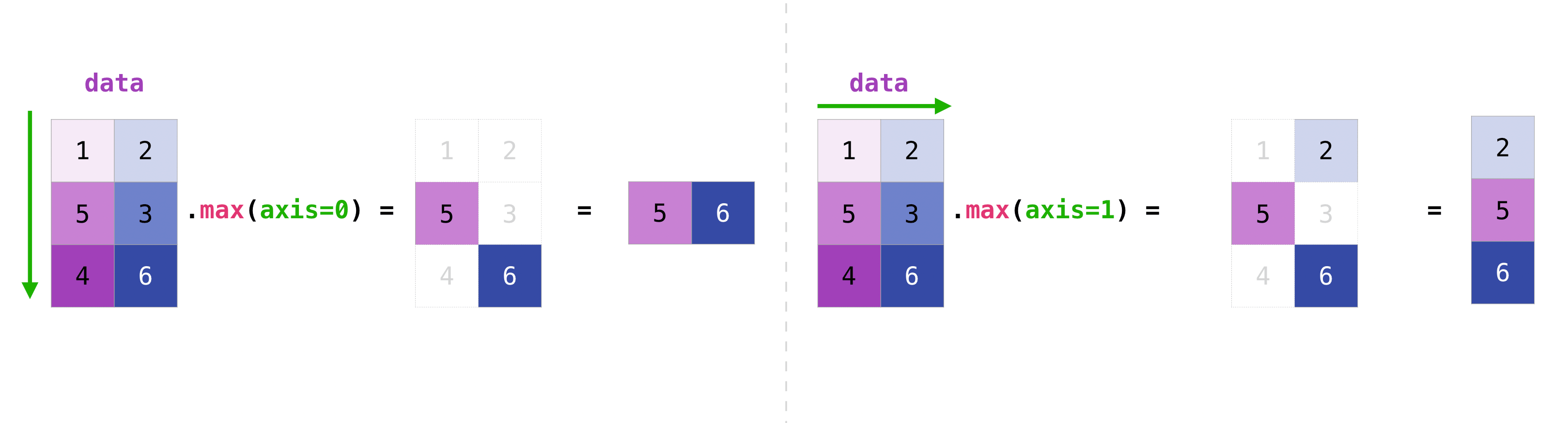
`axis=0` collapses across rows (one result per column); `axis=1` collapses across columns (one result per row).

A_44 = np.arange(1, 17).reshape(4, 4).transpose()
print("A_44:\n", A_44)
print("A_44 shape:", A_44.shape)

print("sum all     :", np.sum(A_44))
print("sum axis=0  :", np.sum(A_44, axis=0))   # collapse rows → one value per column
print("sum axis=1  :", np.sum(A_44, axis=1))   # collapse cols → one value per row
print("min axis=1  :", np.min(A_44, axis=1))   # min of each row

A_44:
 [[ 1  5  9 13]
 [ 2  6 10 14]
 [ 3  7 11 15]
 [ 4  8 12 16]]
A_44 shape: (4, 4)
sum all     : 136
sum axis=0  : [10 26 42 58]
sum axis=1  : [28 32 36 40]
min axis=1  : [1 2 3 4]

The same axis argument works on higher-dimensional arrays.

Q_234 = np.arange(1, 25).reshape(2, 3, 4)
print("Q_234:\n", Q_234)
print("Q_234 shape:", Q_234.shape)

print("min axis=0:\n",   np.min(Q_234, axis=0))       # shape (3, 4)
print("min axis=1:\n",   np.min(Q_234, axis=1))       # shape (2, 4)
print("min axis=2:\n",   np.min(Q_234, axis=2))       # shape (2, 3)
print("min axis=(1,2):", np.min(Q_234, axis=(1, 2)))  # shape (2,) — collapse both dims

Q_234:
 [[[ 1  2  3  4]
  [ 5  6  7  8]
  [ 9 10 11 12]]

 [[13 14 15 16]
  [17 18 19 20]
  [21 22 23 24]]]
Q_234 shape: (2, 3, 4)
min axis=0:
 [[ 1  2  3  4]
 [ 5  6  7  8]
 [ 9 10 11 12]]
min axis=1:
 [[ 1  2  3  4]
 [13 14 15 16]]
min axis=2:
 [[ 1  5  9]
 [13 17 21]]
min axis=(1,2): [ 1 13]

10. Views vs. Copies

Understanding whether an operation returns a view (a window into the same memory) or a copy (a completely new allocation) is critical — accidentally mutating shared data is a common source of hard-to-track bugs in NumPy code.

reshape — returns a view when possible

reshape reuses the same memory buffer and just changes the shape metadata. Modifying the reshaped array therefore modifies the original.

a = np.array([1, 2, 3, 4, 5, 6])
b = a.reshape(2, 3)

b[0, 0] = 999
print("a after modifying b:", a)   # [999, 2, 3, 4, 5, 6] — original changed

print("b.base is a:", b.base is a)  # True → b is a view of a

a after modifying b: [999   2   3   4   5   6]
b.base is a: True

Use .copy() to get an independent array:

c = a.reshape(2, 3).copy()
c[0, 0] = 0
print("a after modifying c:", a)   # unchanged
print("c.base is a:", c.base is a)  # False → c is independent

a after modifying c: [999   2   3   4   5   6]
c.base is a: False

When does reshape return a copy?

If the array is non-contiguous in memory (e.g. after transposing or fancy indexing), NumPy cannot create a view and silently returns a copy instead. You can always check with .base: if it is None, the array owns its data.

Broadcasting operations — always return a new array

A + b, A * b, etc. produce a new array. Modifying the result never affects the original operands.

A = np.arange(6).reshape(2, 3)
b = np.array([10, 20, 30])

result = A + b
result[0, 0] = 999

print("A unchanged:\n", A)
print("b unchanged:", b)

A unchanged:
 [[0 1 2]
 [3 4 5]]
b unchanged: [10 20 30]

In-place operators (+=, *=, …) are the exception — they write directly into the left-hand array:

A_copy = A.copy()
A_copy += b          # A_copy is modified in-place
print("A_copy after +=:\n", A_copy)
print("b unchanged:", b)

A_copy after +=:
 [[10 21 32]
 [13 24 35]]
b unchanged: [10 20 30]

EX) pairwise subtraction

Suppose you have a (3×3) matrix x and a (2×3) matrix y, and you want to subtract every row of y from every row of x, producing a (3, 2, 3) result. Direct subtraction fails because the shapes are incompatible.

x_33 = np.array([[5., 2, 1], [4, 2, 6], [1, 1, 0]])
y_23 = np.array([[1.0, 4, 3], [2, 1, 4]])

try:
    x_33 - y_23
except ValueError as e:
    print("ValueError:", e)

ValueError: operands could not be broadcast together with shapes (3,3) (2,3)

Inserting np.newaxis makes the shapes broadcast-compatible:

# x_33[:, np.newaxis, :] → (3, 1, 3)
# y_23[np.newaxis, :, :] → (1, 2, 3)
# result                 → (3, 2, 3) via broadcasting
z_323 = x_33[:, np.newaxis, :] - y_23[np.newaxis, :, :]
print("result shape:", z_323.shape)
print("row 0 of y subtracted from all rows of x:\n", z_323[:, 0, :])
print("row 1 of y subtracted from all rows of x:\n", z_323[:, 1, :])

result shape: (3, 2, 3)
row 0 of y subtracted from all rows of x:
 [[ 4. -2. -2.]
 [ 3. -2.  3.]
 [ 0. -3. -3.]]
row 1 of y subtracted from all rows of x:
 [[ 3.  1. -3.]
 [ 2.  1.  2.]
 [-1.  0. -4.]]

EX) MSE Loss

The ease of implementing mathematical formulas that work on arrays is one of the things that make NumPy so widely used in the scientific Python community.

For example, this is the mean square error formula (a central formula used in supervised machine learning models that deal with regression):

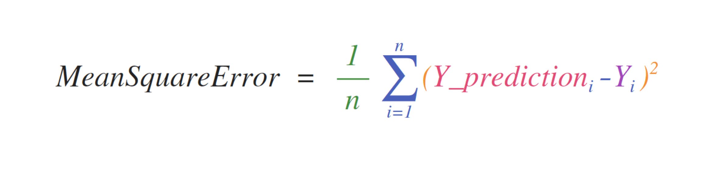
Implementing this formula is simple and straightforward in NumPy:

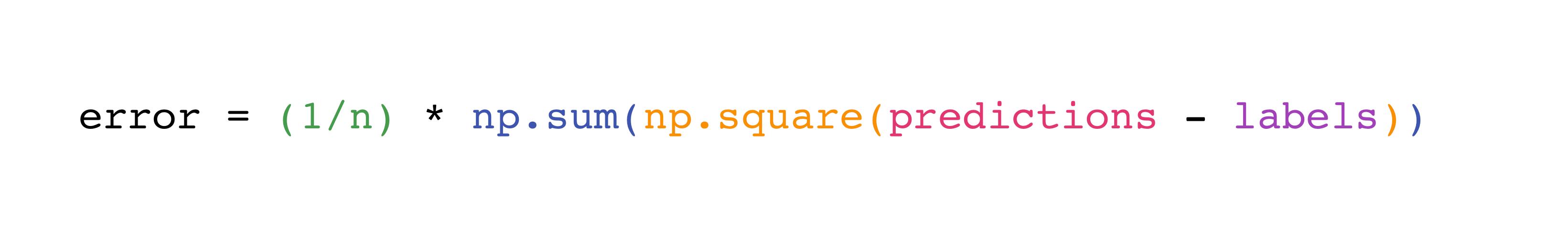
predictions = np.array([1, 2, 3])
labels = np.array([1.5, 2.5, 3.5])

error = (1/len(predictions)) * np.sum(np.square(predictions - labels))
print(error)

0.25

What makes this work so well is that predictions and labels can contain one or a thousand values. They only need to be the same size.

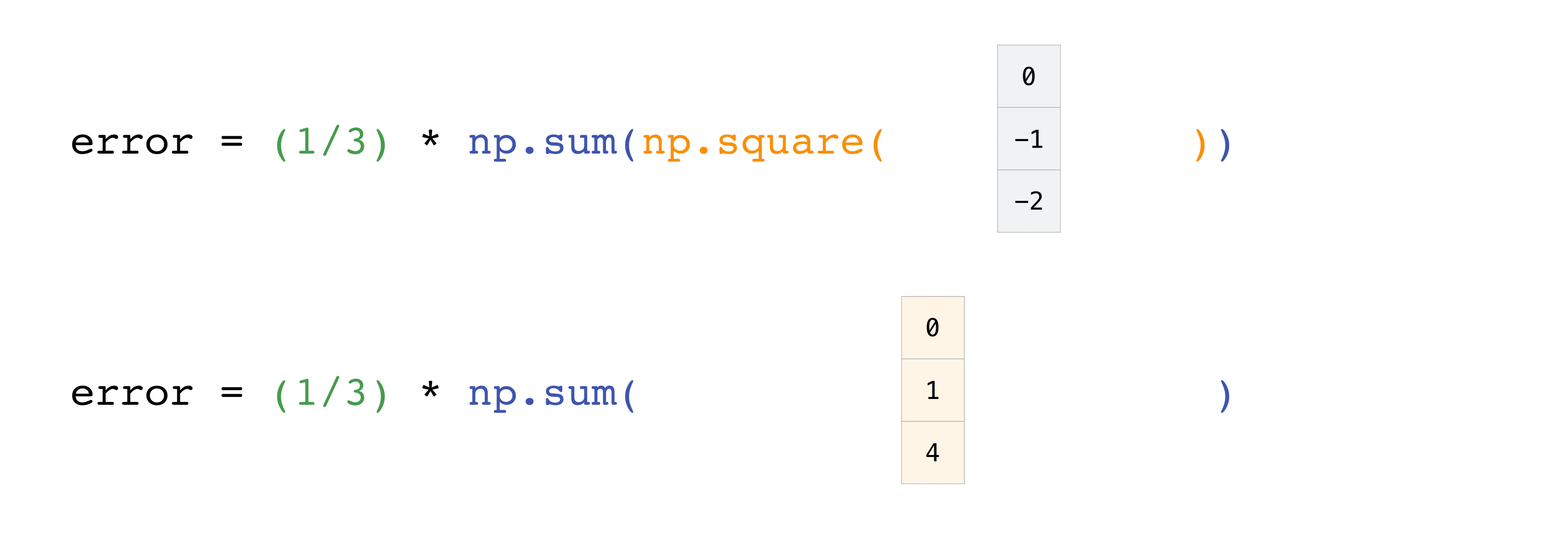
You can visualize it this way:

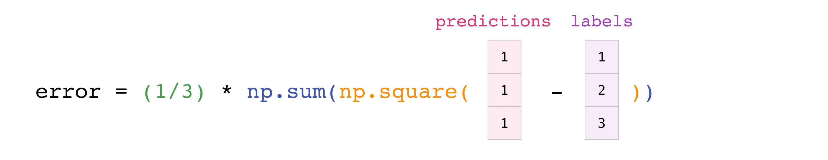
In this example, both the predictions and labels vectors contain three values, meaning n has a value of three. After we carry out subtractions the values in the vector are squared. Then NumPy sums the values, and your result is the error value for that prediction and a score for the quality of the model.

EX) Image Blurring

A single photo (e.g. of a house or street) is just a NumPy array: grayscale images have shape (height, width) and color images (height, width, 3) for red, green, and blue. We will load both versions of the same scene, compare how they are stored, then use sliding local windows over the grayscale image to build a simple blur—each output pixel is the mean of a small square of input pixels. The same idea (local windows over a grid) appears in time series (rolling averages) and in convolutional layers in deep learning.

Loading the image: grayscale and color

We use two files: a grayscale PNG and an RGB PNG of the same scene. The image is of the Lorch Monastery church; the original photograph is available at Wikimedia Commons. Grayscale images give one number per pixel, while RGB images give three numbers per pixel (one for each of red, green, and blue). If your grayscale file is instead stored as three identical channels (R=G=B), we collapse it to 2D so we have a single intensity per pixel.

import io
import urllib.request
import matplotlib.pyplot as plt
import matplotlib.image as mpimg

BASE_URL = "https://raw.githubusercontent.com/GLI-Lab/machine-learning-course/main/data"

def load_image(filename):
    url = f"{BASE_URL}/{filename}"
    with urllib.request.urlopen(url) as response:
        return mpimg.imread(io.BytesIO(response.read()), format="png")

img_gray = load_image("image_gray.png")
img_rgb  = load_image("image_rgb.png")

# If grayscale was stored as 3-channel (R=G=B), collapse to 2D
if img_gray.ndim == 3:
    img_gray = img_gray[:, :, 0]

print("Grayscale shape :", img_gray.shape, "→ one value per pixel")
print("RGB shape       :", img_rgb.shape, "→ three values per pixel")

Grayscale shape : (317, 500) → one value per pixel
RGB shape       : (317, 500, 3) → three values per pixel

fig, axes = plt.subplots(1, 2, figsize=(10, 4))
axes[0].imshow(img_gray, cmap='gray')
axes[0].set_title("Grayscale")
axes[0].axis("off")
axes[1].imshow(img_rgb)
axes[1].set_title("RGB")
axes[1].axis("off")
plt.tight_layout()
plt.show()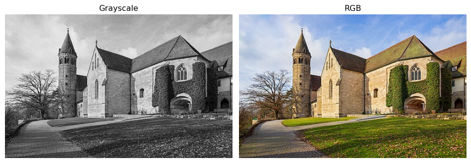

Local windows and simple blur

Replace each pixel by the mean of a small square (e.g. 10×10) around it. That gives a blurred image: edges soften and noise is reduced. We do this by sweeping a sliding window over the array—same idea as a rolling mean along a 1D signal, but in 2D.

A 3×3 window in the top-left corner of the grayscale image looks like this:

top_left = img_gray[:3, :3]
print("Top-left 3×3 block:\n", top_left)
print("Mean of this block:", top_left.mean())

Top-left 3×3 block:
 [[0.85882354 0.85882354 0.85882354]
 [0.83137256 0.83137256 0.8352941 ]
 [0.8235294  0.8235294  0.827451  ]]
Mean of this block: 0.83878

Double loop: For every possible top-left corner (i, j) on the full image, take the block img[i:i+size, j:j+size], compute its mean, and store it. Clear, but many Python iterations.

import timeit

size = 10
m, n = img_gray.shape
mm, nn = m - size + 1, n - size + 1

result_loop = np.empty((mm, nn))
for i in range(mm):
    for j in range(nn):
        result_loop[i, j] = img_gray[i : i + size, j : j + size].mean()

def run_loop():
    r = np.empty((mm, nn))
    for i in range(mm):
        for j in range(nn):
            r[i, j] = img_gray[i : i + size, j : j + size].mean()
    return r
t_loop = timeit.repeat(run_loop, number=1, repeat=10)
print("Loop:       {:.4f} s (mean of 10 runs)".format(np.mean(t_loop)))
print("Blurred shape:", result_loop.shape)

Loop:       0.4018 s (mean of 10 runs)
Blurred shape: (308, 491)

Vectorized view with as_strided: NumPy’s stride_tricks.as_strided lets you reinterpret the same memory as a 4D array of overlapping windows over the full image. No extra memory for the tiles; we only change how we index into the array. Then we take the mean over the last two axes to get one number per window.

from numpy.lib import stride_tricks

shape = (mm, nn, size, size)
strides = 2 * img_gray.strides
windows = stride_tricks.as_strided(img_gray, shape=shape, strides=strides)
result_vec = windows.mean(axis=(-1, -2))

def run_vec():
    w = stride_tricks.as_strided(img_gray, shape=shape, strides=strides)
    return w.mean(axis=(-1, -2))
t_vec = timeit.repeat(run_vec, number=1, repeat=10)
print("Vectorized: {:.4f} s (mean of 10 runs)".format(np.mean(t_vec)))
print("Same as loop:", np.allclose(result_loop, result_vec))
print("Speedup:     {:.1f}x".format(np.mean(t_loop) / np.mean(t_vec)))

Vectorized: 0.0189 s (mean of 10 runs)
Same as loop: True
Speedup:     21.3x

Output comparison: Both methods produce the same blurred image over the full image; the vectorized version is typically much faster.

fig, axes = plt.subplots(1, 3, figsize=(12, 4))
axes[0].imshow(img_gray, cmap='gray')
axes[0].set_title("Original (full image)")
axes[0].axis("off")
axes[1].imshow(result_loop, cmap='gray')
axes[1].set_title("Blurred (loop)")
axes[1].axis("off")
axes[2].imshow(result_vec, cmap='gray')
axes[2].set_title("Blurred (vectorized)")
axes[2].axis("off")
plt.tight_layout()
plt.show()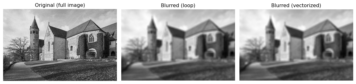

Strides and views

The strides of an array tell how many bytes to skip when moving by one step along each dimension. as_strided only changes the shape and strides; it does not copy data, so you get a new view of the same buffer. For production code, libraries like Scikit-Learn provide helpers to extract sliding windows without writing strides by hand.

Summary

Arrays. NumPy’s ndarray is the universal data container in ML. Every dataset, weight matrix, gradient, and activation tensor is an ndarray. Check shape, dtype, and ndim first whenever you encounter a new array.

Indexing. Use arr[i] for rows, arr[:, j] for columns, arr[a:b, c:d] for submatrices, and fancy indexing arr[[i1, i2]] for arbitrary row selections. Slices return views; fancy indexing returns copies.

Reshaping. reshape and np.newaxis let you add or remove size-1 dimensions without copying data. This is the key to making broadcasting work correctly.

Vectorization and Broadcasting. Never use Python for loops for element-wise array math. NumPy’s C-level operations are orders of magnitude faster. Broadcasting extends operations to arrays of different (but compatible) shapes automatically.

Matrix multiplication. np.matmul (or @) is not element-wise — it computes the standard linear algebra product. Keep the distinction clear: A * B vs A @ B.

Reproducibility. Always seed your PRNG (np.random.RandomState(seed)) before generating any random data used in training or evaluation.

Reductions. np.sum, np.min, np.max, np.mean with an explicit axis argument are the standard way to aggregate over samples, features, or time steps without writing loops.